If you work in IT, learn how BetterCloud’s Unified SaaS Management platform can help you manage G Suite and other applications. Also, learn how you can 10x your G Suite productivity. 

Applying some color to alternating rows in a spreadsheet can make it easier to read. Of course, you could manually change the background color of columns or rows, but who has time for that? So here’s how to use conditional formatting to automatically create a colorful and attractive spreadsheet in Google Sheets.

• In Google Sheets, head up to Format and click on Conditional formatting.
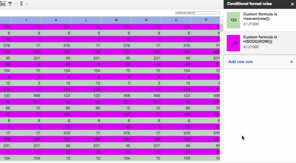
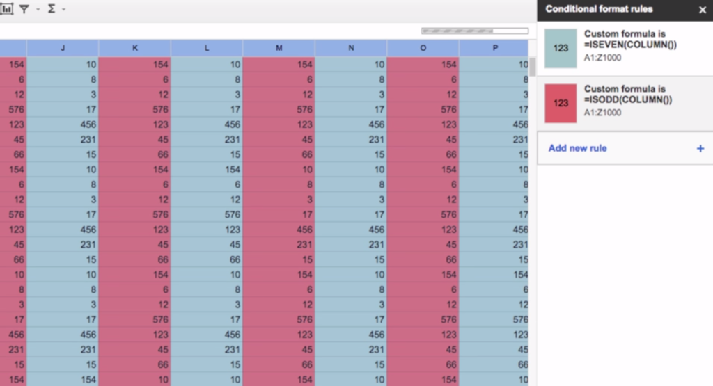
• Select “Add new rule.” Select the range using the “Apply to range” field, and then under the “Format cells if…” dropdown menu, select “Custom formula is.” Then, there are four basic rules you can create here to dictate how and where you’d like color applied to your sheet.
• To apply a color to all even rows, type =ISEVEN(ROW()). To apply the rule to odd rows, type =ISODD(ROW()). Click the paint bucket icon to change the color.

• To apply color to all even columns, type =ISEVEN(COLUMN()). To apply the rule to odd columns, type =ISODD(COLUMN()).

Click here to watch this video on YouTube.