In part four of our miniseries on the most popular Excel functions, we’ll cover the “VLOOKUP” function, which is very useful for finding specific information in your worksheet.

If you missed it, check out part one (“IF”), part two (“SUM”), and part three (“COUNTIF”) of our series.

VLOOKUP is short for vertical lookup. It’s a little more complicated than some of the functions that we’ve looked at previously in the series, because this time, there are four different values within the function that you need to input.

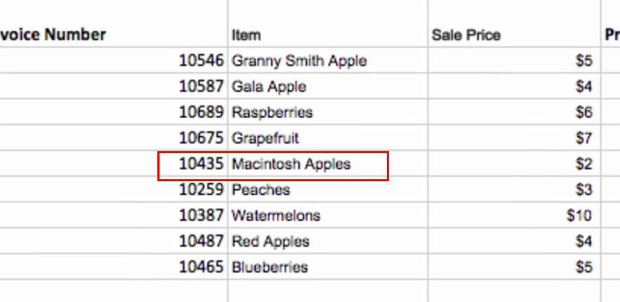
So as you can see here, we have a simple form keeping track of fruit we’ve ordered for our fictional store. In this example, we’re going to search for an invoice number and find the corresponding item the invoice is for. VLOOKUP works like this: It will search vertically down a column for the specified invoice number, and once it finds it, it moves to the next column to return the corresponding value (the fruit).

 

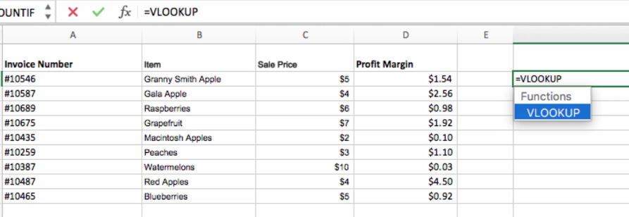
To show you how this works, we’re going to start by entering =VLOOKUP and then opening parentheses.

 

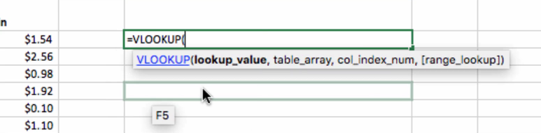
Now, the first term that we need to enter is the lookup value – this is the item that we’re going to search for in the first column of the table in question. So, we’re going to enter in the invoice number (10435) that we’re searching for here.

 

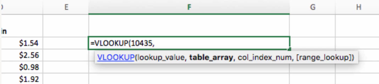
Next, we’re going to put a comma to separate our terms, and now we have to specify the table that we want included in our search with the function. So the easiest way to do that is to just drag and select the table that you want included, and then insert a second comma.

 

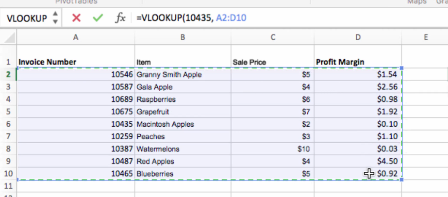
The next number is going to indicate the column in the selected table that we want to pull the value from after locating the value we’re searching for. So since the first column in the table is always 1, then we want to return the value from column 2, since we want the type of fruit the invoice corresponds with.

 

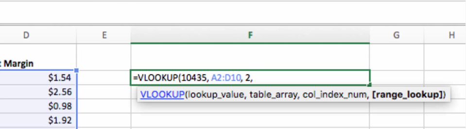
The final term we need to include is the approximate match, which determines whether you have to have an exact or approximate match of the value specified in order to return a lookup value. It will be either TRUE or FALSE. In this case, we’re going to say FALSE, which indicates that an approximate match is not allowable.

 

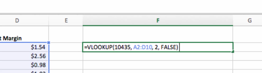
And when we hit Enter, the result we get is Macintosh Apples.

Since our invoice number was found in column A, it returned the corresponding value from column B. 

 

The VLOOKUP function can be useful because you can pull in values from other sheets as well. You can specify that you want to pull a value from another sheet, and VLOOKUP will bring it into your new sheet.

 

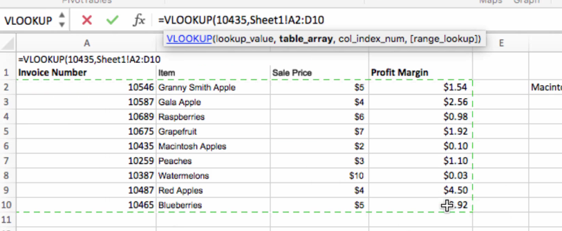
You can even access other workbooks this way, which is one of the most valuable applications of the VLOOKUP function – it gives you a tool to integrate data across multiple sheets and workbooks as you may require.

Click here to watch this video on YouTube.