How to Use Icons in Your Conditional Formatting in Excel for Mac

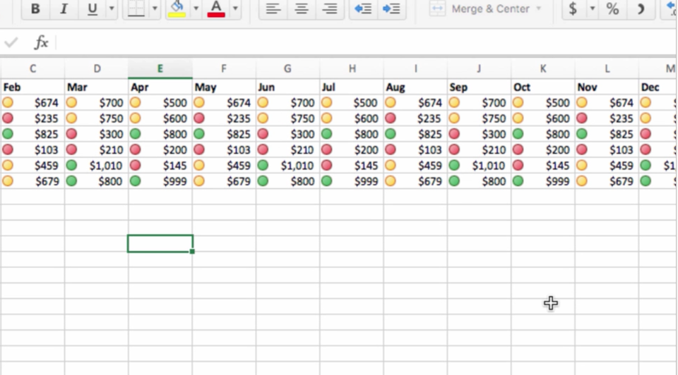
You might already know how to use conditional formatting in Excel, but you can use icon sets to make it even more visually powerful. These icons correspond to your conditional formatting and they come in a variety of colors and shapes (stars, flags, traffic lights, etc). By using them in your spreadsheets, you can instantly highlight patterns and trends in your data.

To apply conditional formatting, first select all of the data that you want to apply your formatting rule to. Click on Format > Conditional Formatting.

The conditional formatting dialogue box will open up. Click on the + icon in the lower left-hand corner, which will allow you to add a new formatting rule to the spreadsheet.

This next box is where you’ll set the terms of your formatting. So, in order to apply icons, go to the Style dropdown menu and select Icon Sets.

Under the dropdown menu labeled Icons, you can see the various icon sets you can apply to your formatting. There are shapes like arrows, flags, traffic lights, stars–you name it. These are great because they represent data in a very visual way that anyone can quickly understand. It can even be useful for surpassing language barriers. Select a set that you like.

You can set how these icons will be applied. The dropdown menus allow you to select when the rule will be applied, and whether you want it applied based on number, percent, formula, or percentile. You can enter specific values in the boxes as well.

You can also create custom icon sets using the “Display” dropdown menus. The “Show icon only” box allows you to display only the icon, which will remove the original data from the conditional formatting view.